Basic Principle of OFDM Technology

Abstraction

In this project, we focus on learning how to solve the problem of inter-symbol interference using OFDM techniques. We applied the properties of periodic convolution and DFT to process the signal and perfectly avoid the disadvantage of DTFT which cannot be processed by computer because it is continuous. After we designed the whole system of OFDM, we also simulated the whole process by passing random signals. From the whole project, we learned that transmitting signals in the frequency domain is much better than transmitting them in the time domain in terms of avoiding signal delay diffusion.

Introduction

Baseband of OFDM

Block 1:

A sequence data:

After Serial-to-Parallel Converter:

They will be packaged into:

Via IFFT,

In order to weaken the influence of both ISI and ICI and gain the correct information after FFT and IFFT, cyclic prefix (CP) is required. The length of CP supposed to be M, is associated with the length of delay.

Block 2:

After transmission:

To obtain the valid information, we need remove CP from the signal first:

The Serial-to-Parallel Converter helps FFT operate. Then we get:

By being dividing by $N \widetilde{H}[i]$,

Now we can obtain the original sequence $\{a_n\}$ by the Parallel-to-Serial Converter.

DAC + RF front-end of the transmitter

DAC is:

$\mathcal{R} e\left\{x_{c}(t)\right\}$ and $\mathcal{I}m\left\{x_{c}(t)\right\}$ are used to modulate the amplitude of orthogonal functions $\cos \left(n \omega_{c} t\right)$ and $\sin \left(n \omega_{c} t\right)$, $\omega_{c}=\frac{2 \pi}{T}$.

Sum all OFDM signals,

Receiver Design and Analysis

Task A: Receiver RF front-end + ADC

To demodulate the signal, we multiply $\cos(\omega_c t)$ and $\sin(\omega_c t)$.

Calculate the average signal in a length of a period.

Similarly,

After multiply $\mathcal{I} m\left\{x_{k}^{\prime}[n] * h[n]\right\}$ with $j$， we have the output.

Task B: The Relation between h(t) and h[n]

We know the impulse response of actual wireless channel is:

Then we change it to DT signal:

So,

Task B: The length of CP

Prefixing it with a cyclic prefix of length M, the OFDM symbol obtained is:

Assume that the channel is represented using

Then, after convolution with the channel, which happens as

So, taking the Discrete Fourier Transform, we get

Thus, a multipath channel is converted into scalar parallel sub-channels in frequency domain, thereby simplifying the receiver design considerably.

We can find that if we take $M=\rm length(h[n])-1$, we can get the same result as period convolution. However if $M<\rm length(h[n])-1$, we cannot get the same result.

So, the length of CP is length of h[n] - 1 = 3.

Simulation

Initialize

n_channel = 32; n_data = 64; m_cp = 3; R = 1000; 
wc = 1e11 / R; 
n_seq = n_channel + n_data;
n_bits = ceil(n_seq / n_channel);
n_train = n_bits * (n_channel + m_cp);

pilot = ones(1, n_channel);
data_tx = randi([0, 1], 1, n_data);

Block 1

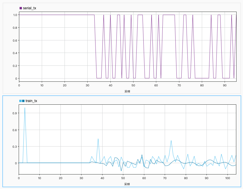
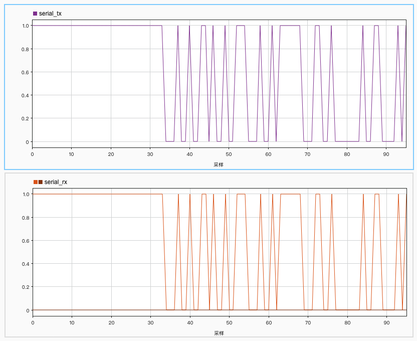
serial_tx = [pilot data_tx];
parallel_tx = reshape(serial_tx, n_channel, n_bits);
ftseq_tx = zeros(n_channel, n_bits);
for i = 1 : n_bits
    ftseq_tx(:, i) = ifft(parallel_tx(:, i));
end
dtseq_tx = zeros(n_channel + m_cp, n_bits);
for i = 1 : n_bits
    CP = ftseq_tx(n_channel - (m_cp-1) : n_channel, i);
    dtseq_tx(:, i) = [CP; ftseq_tx(:, i)];
end
train_tx = reshape(dtseq_tx, [1, n_train]);

Block 3

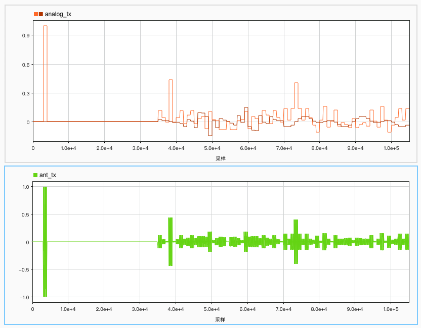
analog_tx = repelem(train_tx, R);
t_tx = 0 : R * n_train - 1;
cos_tx = cos(wc .* t_tx);
sin_tx = sin(wc .* t_tx);
ant_tx = real(analog_tx) .* cos_tx + imag(analog_tx) .* sin_tx;

Transmit

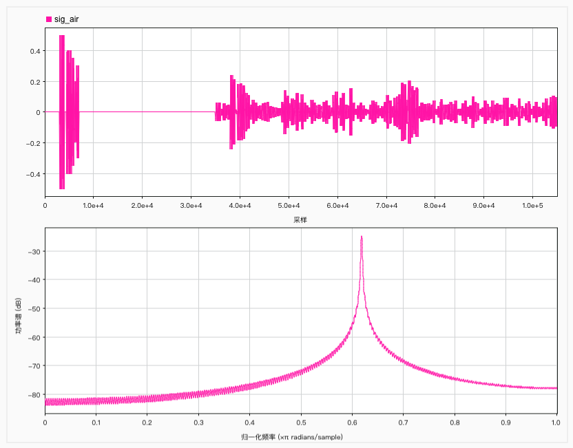
h = [0.5 zeros(1, 1.5 * R - 1) 0.4 zeros(1, R - 1) ...
    0.35 zeros(1, 0.5 * R - 1) 0.3];
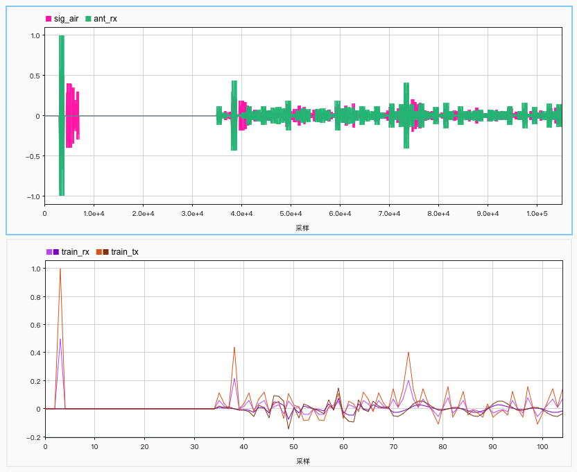
sig_air = filter(h, 1, ant_tx);

Block 4

ant_rx = filter(1, h, sig_air);
t_rx = 0 : length(ant_rx) - 1;
cos_rx = cos(wc .* t_rx);
sin_rx = sin(wc .* t_rx);
real_rx = ant_rx .* cos_rx;
imag_rx = ant_rx .* sin_rx;
train_rx = zeros(1, n_train);
for i = 1 : n_train
    train_rx(i) = mean(real_rx((i - 1) * R + 1 : i * R)) ...
        + 1j * mean(imag_rx((i - 1) * R + 1 : i * R));
end

Block 2

parallel_rx = zeros(n_channel, n_bits);
for i = 1 : n_bits
    parallel_rx(:, i) = 2 * train_rx((i-1) * (n_channel + m_cp) ...
        + (m_cp + 1) : i * (n_channel + m_cp));
end
ftseq_rx = reshape(parallel_rx, 1, n_seq);
serial_rx = zeros(1, n_seq);
for i = 1 : n_bits   
    serial_rx((i-1) * n_channel + 1 : i * n_channel) = ...
        fft(ftseq_rx((i-1) * n_channel + 1 : i * n_channel));
end

Discussions

The technical advantages of OFDM are as follows:

1. High resistance to frequency selective fading or narrowband interference. In a single-carrier system, a single fading or interference can cause the failure of the entire communication link, but in a multi-carrier system, only a small fraction of the carriers will be interfered with.OFDM transmits user information through multiple subcarriers, and the signal time on each subcarrier is many times longer than that on a single-carrier system at the same rate, making OFDM more resistant to impulsive noise and fast fading channels. Also, the resistance to impulsive noise and fast fading of the channel is enhanced by the joint coding of the subcarriers, which achieves frequency diversity among the subchannels.
2. Strong ability to resist ISI and ICI. OFDM has a strong ability to resist intercede interference due to its protective spacing and cyclic prefixes.
3. High frequency utilization. OFDM allows overlapping common subcarriers to be used as subchannels, allowing a large amount of data to be transmitted in a narrowband bandwidth. It saves nearly half of the bandwidth compared to conventional FDM techniques and improves frequency utilization efficiency by using a protected-band approach to splitting subchannels.
4. High channel utilization rate. When the number of subcarriers is large, the spectrum utilization of the system tends to 2Baud/Hz.
5. The implementation of OFDM technology is relatively easy. The implementation method of OFDM can be chosen between IFFT/FFT.
6. Suitable for high-speed data transmission. OFDM enables different sub-carriers to be modulated in different ways under the transmission medium, depending on the channel conditions and noise background, and automatically detects which particular carrier has high signal attenuation or interference pulses. When the channel conditions are good, the modulation method with high efficiency is used. When the channel conditions are poor, the modulation method with high anti-interference capability is used. In addition, the OFDM loading algorithm is used to enable the system to put more data in a channel with good conditions and transmit at high speed. Therefore, OFDM technology allows dynamic adaptation to turn on and off the corresponding carriers to ensure continuous and successful communication, which is ideal for high-speed data transmission.